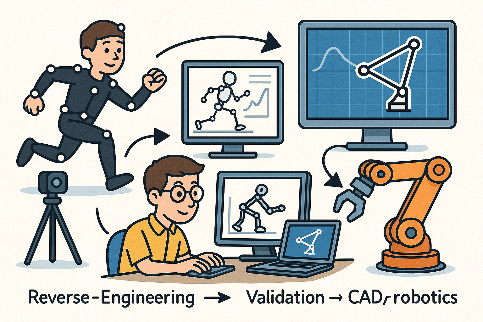
Reverse-Engineering Mechanisms from Motion Capture: Kinematic Identification, Validation, and CAD/Robotics Export

Why reverse-engineer assemblies from motion capture and kinematics

Strategic value

Reverse-engineering assemblies directly from measured motion offers a decisive path to understanding complex mechanisms without teardown, revealing the design intent that lives in constraints rather than in static geometry. By capturing how parts actually move and interact, teams uncover the implicit kinematic architecture—the axes, limits, and couplings—that define function, tolerance budgets, and failure modes. The immediate advantages span competitive analysis, brownfield modernization, and human-centered devices. You can digitize legacy machinery and competitor products without disassembly, using multi-view video or marker-based MoCap to infer the joint graph and parameters, even when CAD is unavailable or deliberately obfuscated. You can accelerate fixture and automation design by extracting real joint behavior from shop-floor videos, turning quick phone captures into measurable axes and travel that inform grippers, nests, and guards. You can close the loop between field performance and CAD by capturing wear, backlash, and misalignment, comparing simulated vs observed trajectories to localize drift to specific constraints. And you can translate biomechanical motion into engineered mechanisms for exoskeletons and prosthetics, mapping anatomical kinematics to practical linkages with manufacturable joints and adjustable compliance. The outcome is a living, measured assembly that supports simulation, off-the-shelf mechanism selection, and limits/clearances that hold up under production variability.

• Minimal intrusion: no teardown, no safety barrier removal, minimal downtime.
• Design-speed feedback: quantify where range, backlash, or stiction truly are limiting throughput.
• Evidence-guided tolerancing: distribute clearances where they reduce cumulative error most.
• Human-in-the-loop motion capture that directly informs mechanism synthesis for assistive devices.

Scope and assumptions

To make the approach tractable and repeatable, most pipelines target rigid-body mechanisms with standard joints—revolute, prismatic, planar, cylindrical, helical, and spherical. This assumption covers the overwhelming majority of industrial mechanisms, machine-tool stages, robotics wrists, latches, hinges, and sliders. While many real systems are slightly compliant, treating links as rigid with small elastic byproducts is often sufficient for kinematic identification; compliance can be estimated separately as a low-order correction. On the sensing side, robust pipelines accept heterogeneous data sources: optical MoCap (marker-based or markerless), video SLAM, IMUs, and robot logs. Marker-based capture with triads or asymmetric constellations remains the gold standard when access is possible; markerless MoCap and video SLAM shine when the system cannot be instrumented. IMUs help bridge occlusions and stabilize orientation estimates, and robot controller logs provide joint-angle ground truth that can anchor multi-sensor fusion. Practical assumptions include reasonably persistent excitation, manageable occlusion rates, and the ability to establish a global scale and time synchronization. Within that envelope, you can recover joint topology, limits, offsets, and key non-idealities and export them as mates that rebuild in major CAD and robotics packages.

• Rigid links, small motion-induced compliance modeled as a perturbation.
• Standard joint taxonomy; non-standard contacts treated as intermittent constraints.
• Accept mixed-modality data; solve in a common frame with known or estimable scale.
• Moderate lighting/texture suffices for markerless; markers or fiducials reduce ambiguity.

Success criteria

Reliable reverse-engineering demands metrics that reflect both graph structure and geometric precision, as well as how well the inferred mechanism replicates observed motion. Start with joint-type classification accuracy and assembly graph correctness, reported via precision/recall or F1 scores against known ground truth or expert-reviewed labels. Next, quantify parameter error with axis orientation/position RMSE in the world frame, joint limit error in degrees or millimeters, and data-driven backlash estimates derived from direction-dependent hysteresis loops. Evaluate replay fidelity by driving a multibody simulation with the inferred parameters and comparing reprojected trajectories to the recordings; report per-point or per-body reprojection error and loop-closure drift over time. Finally, check export quality: do mates rebuild robustly in the target CAD? Are constraints minimized and named consistently? Do joint limits and offsets load into URDF/SDF without warnings? A rigorous pipeline treats these metrics as gates, not suggestions, and maintains dashboards so engineers can triage where inference fails—classification confusion, insufficient excitation, or scale/time misalignment—and plan the next capture iteratively for maximal learning and minimal recapture effort.

• Topology: F1 ≥ 0.9 for joint types and adjacency under representative captures.
• Geometry: axis direction RMSE ≤ 1–2°, axis location RMSE ≤ 1–2 mm with proper calibration.
• Backlash bounds: repeatable deadband estimates within ±10% across cycles.
• Replay: reprojection error near sensor noise floor; loop-closure residuals stable over time.
• Export: mates load without overconstraints; naming reflects design intent (e.g., “Door_Hinge_Axis”).

Data capture and preprocessing that make kinematic inference robust

Instrumentation and calibration

High-quality inference begins with disciplined sensing. Calibrate multi-camera rigs thoroughly: intrinsic/extrinsic parameters, lens distortion models, and vignetting if photogrammetry is involved. For time alignment across cameras and inertial sensors, pursue PTP or IR strobe synchronization so motion discontinuities do not masquerade as backlash. When you can instrument the mechanism, adopt a marker strategy that uses rigid triads or asymmetric constellations per rigid body to lock the body’s pose unambiguously; avoid symmetric point layouts that increase label confusability. For hard-to-stick surfaces, mount small plates with fiducials such as ArUco or AprilTags to create high-contrast, quickly localizable targets. Wherever occlusions are likely—inside guards, under carriages, behind operators—hybridize with sparse IMUs on the most occlusion-prone bodies; even a few gyros can stabilize orientation around challenging axes. If the mechanism already contains encoders or a robot controller exposes joint angles, tap those logs to anchor relative phase and scale. The goal isn’t maximal sensor count; it’s a balanced set that sees each body in motion with stable reference overlap, consistent scale, and verified timing. A brief pilot capture that stresses known pain points will almost always pay back many hours of post-processing.

• Board-lens calibration for each camera, then stereo/array extrinsics; verify reprojection RMS.
• Sync verification via flashing beacon or shaker to check sub-millisecond alignment.
• Marker IDs printed with non-repeating geometry; place on faces with varied normals.
• Use magnet or adhesive plates with fiducials to survive heat, oil, and vibration.
• Add IMUs to bodies that rotate out of view; align frames during preprocessing.

Excitation design (identifiability)

Even the best sensors can’t rescue an uninformative motion script. Design excitation for identifiability: isolate degrees of freedom before combining them, sweep velocities and directions, and deliberately cross known transition points to expose backlash and stiction. Exercise one DOF at a time when possible, then follow with multi-DOF sweeps that explore combinations. For prismatic joints, execute spiral or raster motions across the plane orthogonal to the suspected axis so translation directions span a rank-1 subspace along the guide; for revolute joints, command large rotations about the suspected axis while creating off-axis lever arms to condition axis location. Vary the velocity profile and reverse direction to capture hysteresis; pause at end-stops to bound limits and observe settle behavior. In closed chains, ensure persistency of excitation over the loop; if safe, temporarily break loops or reduce constraints so individual pairs can be excited without compensation couplings that obscure the joint classification. A short, well-planned script—minutes, not hours—yields relative motions rich enough to support robust screw-fitting, while minimizing fatigue for human-in-the-loop captures and reducing cycle disruption on the factory floor.

• Scalar sweeps for sliders; large-amplitude arcs for hinges; mixed paths for planar joints.
• Bidirectional passes across backlash; slow ramps to separate viscous vs Coulomb friction.
• Occasional taps at limits to log contact normals and offsets for stop geometry.
• Closed-loop mechanisms: excite independent loops sequentially; lock known DOFs if needed.

Signal conditioning

Raw tracks are not poses. Convert detections into smooth, physically consistent SE(3) trajectories for each body and align them in a common world. Start with rigid-body clustering: group markers by low inter-point distance variance over time; reject points whose pairwise distances drift beyond a small threshold. Estimate per-body pose using absolute orientation methods or PnP for fiducials, then smooth with a Savitzky–Golay or Butterworth filter tuned to preserve real dynamics without phase-lagging joint reversals. Outliers are inevitable, so use RANSAC for each pose solve across short windows and fill gaps with Kalman smoothing or factor-graph optimization that couples bodies via soft constraints. Resolve global frame alignment early: define a world datum with a surveyed plate, a known hinge axis, or gravity alignment; if data are monocular or SLAM-derived, explicitly solve scale via a known baseline such as a tagged caliper bar. Time synchronization should be revisited post-hoc by maximizing cross-correlation of independent orientation channels; even small drifts can bias backlash estimates. The output of conditioning is a set of timestamped, uncertainty-aware poses with consistent scale and minimal bias—suitable for relative motion analysis and the screw-theoretic tests that power classification.

• Pose smoothing with uncertainty propagation; avoid over-smoothing around reversals.
• Windowed outlier rejection; reweight by per-marker covariance from detection confidences.
• Datum enforcement: fix one body as ground; maintain a repeatable XYZ convention.
• Sensor fusion that respects different noise spectra for video vs IMUs.

From motion to assembly: algorithms, export, and pitfalls

Pairwise joint-type inference

With body trajectories in hand, the heart of inference is analyzing relative motion between body pairs through the lens of screw theory. Compute instantaneous twists in se(3) by differentiating relative poses or fitting short-window motions, and test hypotheses for each standard joint. For revolute joints, the signature is rotation about a fixed line in space with negligible translation along the axis; estimate the instantaneous screw axis via SVD on relative velocities and fit a Plücker line that remains stable across time windows. For prismatic joints, translation spans a rank-1 translational subspace with minimal rotation; fit a direction in R3 and verify small rotational residuals. Helical joints show coupled rotation and translation with constant pitch; regress translation vs angle and check linearity and residual variance to find the pitch. Planar, cylindrical, and spherical joints can be discriminated by rank tests on velocity/position residuals and by examining the dimension of the constraint manifold implied by the motion. Make the pipeline robust: perform RANSAC across time windows, reweight by measurement covariance, and explicitly test degeneracies (nearly parallel axes, near-planar motions) with conservative priors. Where classification confidence is low, retain multi-hypotheses with scores rather than forcing a brittle single label; the global graph solver can later arbitrate.

• Relative twist estimation with windowed least squares and noise-aware weighting.
• Axis location from point-line distances minimized over all marker trajectories.
• Helical pitch via robust regression; reject outliers from stick-slip reversals.
• Constraint rank tests: dimension counting on velocity Jacobians and pose dispersions.

Assembly graph synthesis

After scoring pairwise joints, assemble a mechanism that is minimal yet consistent. Build a weighted graph whose nodes are bodies and whose edges are candidate joints labeled with types, parameters, and confidence scores. Select a spanning set that connects all bodies with the correct total degrees of freedom; treat extra high-confidence edges as potential loop closures. For mechanisms with kinematic loops, switch to nonlinear least squares or factor-graph optimization (e.g., GTSAM): define variables for joint parameters (axis orientation/position, limits, offsets, clearances) and body poses across time, and minimize a global cost that includes reprojection residuals, joint-constraint residuals, and priors from engineering judgment or catalogs. Loops are not a nuisance—they are information: they regularize axes against drift, reveal parallelism or perpendicularity constraints, and expose small clearances. Joint limits and backlash emerge naturally when residuals differ under direction reversals; encode them as asymmetric deadbands and preload states. When multiple joint types explain the data similarly, prefer the simpler type unless residuals demand complexity; document alternative edges as suppressed features for later activation. The solver’s end product is a consistent assembly graph with confidence-weighted parameters that explain the data and are stable under re-simulation.

• Graph search to choose a minimally overconstrained joint set; penalize redundant mates.
• Bundle adjustment flavor factor graphs: poses, axes, and limits co-estimated.
• Parameter uncertainty quantified; store covariances for downstream tolerance analysis.
• Automatic naming and grouping that map cleanly to CAD mates and simulation joints.

Beyond basic joints

Real mechanisms include intermittent contacts, power transmission, and flex that blur the rigid-joint idealization. Enrich the model with detectors for contacts, gears, and cams by correlating collision proximity with velocity screw relations. Gear ratios surface from angular velocity ratios that are stable across load; phase lags expose belt stretch. Cams can be recognized by the evolution of surface normal curvature and a consistent normal alignment between follower and track, visible when motion is reprojected onto candidate contact surfaces. Meanwhile, introduce measured compliance: small elastic deformations appear as low-frequency deviations from rigid kinematics and can be modeled per joint or per link, then flagged as “flexible” for downstream FEA co-analysis. Keep these enrichments modular; the core rigid graph should stand on its own, with contact/coupling elements toggled on to improve replay fidelity only where evidence supports them. The litmus test remains the same: do these additions reduce residuals materially and consistently across repeats without overfitting to one capture? If yes, export them as couplers, gear mates, or spring-damper elements with parameters and confidence bounds.

• Detect gear pairs by stable angular velocity ratios; verify diametral pitch from geometry when available.
• Identify cam followers by consistent normal contact and curvature-driven normal acceleration.
• Model compliance as linear springs/dampers first; escalate complexity only if warranted.

Toolchain and deliverables

Deliverables matter because they carry measured intent into daily tools. Provide mechanism exports in robotics and CAD-native formats, validations that inspire trust, and dashboards that catch regressions early. For robotics, generate URDF/SDF with joint hierarchies, limits, and inertial stubs; for CAD, drive direct mates via APIs (revolute/slider/planar/cylindrical/spherical) with named references and mates grouped logically by subassembly. If a CAD target lacks a full constraint mapping, pair STEP AP242 for geometry with an external JSON/XML file that lists mates, frames, and limits, plus optional contact/coupling elements; include coordinate transforms for frame alignment. Validate by replaying recorded joint trajectories in a multibody solver (Drake or Pinocchio) and comparing reprojected tracks to the raw measurements; publish metrics dashboards that show joint residual norms, axis drift over time, loop-closure error, and per-camera reprojection error distributions. Finally, document practical pitfalls that either require recapture or reparameterization: occlusions and label swaps that destabilize body identification; flexible or belt-driven subsystems masquerading as joints; under-excitation causing misclassification; synchronization drift that inflates backlash; monocular scale ambiguity; and degeneracies from ambiguous parallel axes or near-planar motion. Proactively recommend targeted recapture scripts to resolve ambiguity—e.g., introduce out-of-plane motion or temporary markers—and keep a change log between inference runs so engineers can track exactly what improved and why.

• Exports: URDF/SDF with consistent link frames; CAD mates created with stable references.
• Neutral pairing: STEP AP242 + JSON mates for toolchains without native kinematic import.
• Verification: A/B replay in Drake/Pinocchio with the same excitation; watch loop-closure trends.
• Dashboards: confidence scores, axis drift plots, reprojection histograms per view.
• Pitfalls: occlusion, flexible elements, under-excitation, sync drift, scale, and degeneracies.

Conclusion

Practicality through rigor

Reverse-engineering assemblies from motion has crossed from curiosity to capability because capture has matured, screw-theoretic classification is now routine, and global optimization enforces consistency across loops and time. The practical recipe is straightforward but uncompromising: instrument and calibrate to a standard that keeps reprojection errors at the noise floor; design excitation to make the data speak; condition signals so each body trajectory is smooth, time-aligned, and scaled; and only then fit joints with tests that align with the physics of revolute, prismatic, planar, cylindrical, helical, and spherical constraints. The final mechanism is not a static drawing but a data-backed model that reproduces the observed motion with quantified uncertainty, carries limits and backlash that reflect reality, and integrates cleanly with CAD and simulation. That is what turns a noisy phone video or a handful of markers into a trusted digital assembly. The payoff is immediate: design changes become grounded in measurements, not hunches; validation is automated and objective; and stakeholders can iterate with confidence, knowing that every constraint and limit has been earned by data.

ROI through identifiability and clean export

The highest return on investment consistently comes from pairing smart identifiability-driven experiment design with robust inference and meticulous export that preserves design intent. A capture that excites each DOF separately, sweeps velocities both ways, and briefly kisses end-stops will reveal joint types and limits more reliably than an hour of casual operation. A pipeline that propagates uncertainty, retains multi-hypotheses, and leans on factor-graph solvers to arbitrate loops will reduce rework. And an export that uses minimal, meaningful mates—named by function not geometry—and clean URDF/SDF links accelerates downstream use across CAD, robotics, and CAE. Add to this a habit of closing the loop: replay inferred models against new runs, monitor replay fidelity, and flag drift early. Teams that treat capture → inference → validation → export as a single continuous process find that design reviews, supplier negotiations, and maintenance planning all get simpler because everyone can point to the same, measured assembly instead of debating interpretations of legacy drawings or tribal knowledge.

Near-term advances

The next wave will compress timelines and widen applicability. Expect geometric deep learning to learn joint proposals directly from video and point trajectories, seeding graph construction with high-quality priors that classic tests then verify. Factor-graph solvers will move toward real-time loop closure, allowing on-site validation that a capture has sufficient excitation and that the graph is identifiable before teardown or reassembly proceeds. Learning-assisted detectors for non-idealities—backlash, compliance, stiction—will trigger targeted recapture steps on the spot and quantify changes across maintenance cycles, closing the gap between design and condition monitoring. Improved cross-tool standards will make export quality less brittle: richer URDF/SDF variants, CAD mate ontologies, and AP242 extensions for kinematics and contacts. And lightweight, battery-powered fused sensor rigs—hybrid visual-inertial capture with synchronized coders—will reduce setup costs further, making ad hoc studies on live equipment safe and routine. The common thread is automation with accountability: faster, yes, but also with uncertainty that travels and metrics that remain legible to the engineer in the loop.

Standardized pipelines

As teams converge on standardized capture → inference → validation → export pipelines, noisy field motion will reliably become parametric assemblies that rebuild, simulate, and manufacture cleanly. Templates will encode best practices for calibration, marker placement, and excitation; processing batteries will bake in clustering, pose smoothing, axis fitting, and graph optimization with sensible defaults; and exporters will target the prevailing CAD and robotics ecosystems with minimal friction. On top of these rails, each organization can add its domain specifics—preferred mates, tolerancing schemes, controller interfaces—without reinventing the fundamentals. The result is compounding leverage: every capture improves the shared models and checklists; every verification dashboard tunes thresholds and alerts; and every export enriches the library of constraints that express real-world function succinctly. When that happens, the question shifts from “Can we reverse-engineer this?” to “Which design choice does the data recommend?”, and the answer is delivered not as a diagram but as a working, measurable assembly with clean constraints and mates that survive change, serve simulation, and accelerate production.