Customer Testimonials

"Great customer service. The folks at Novedge were super helpful in navigating a somewhat complicated order including software upgrades and serial numbers in various stages of inactivity. They were friendly and helpful throughout the process.."

Ruben Ruckmark

"Quick & very helpful. We have been using Novedge for years and are very happy with their quick service when we need to make a purchase and excellent support resolving any issues."

Will Woodson

"Scott is the best. He reminds me about subscriptions dates, guides me in the correct direction for updates. He always responds promptly to me. He is literally the reason I continue to work with Novedge and will do so in the future."

Edward Mchugh

"Calvin Lok is “the man”. After my purchase of Sketchup 2021, he called me and provided step-by-step instructions to ease me through difficulties I was having with the setup of my new software."

Mike Borzage

Chance-Constrained Toolpath Planning: Noise-Aware CAM for High-Speed Milling

March 26, 2026 14 min read

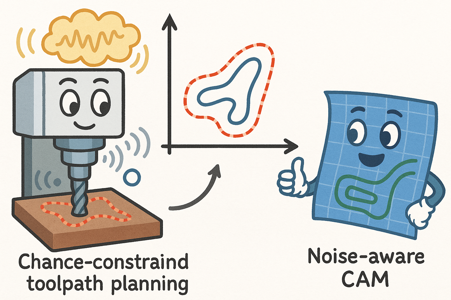
The problem space

Why small disturbances become big at high-speed

At the feeds, accelerations, and spindle speeds of high-speed milling (HSM), tiny disturbances propagate through the kinematic chain and are multiplied by structural dynamics. A few microns of **servo lag**, a few micrometers of **spindle runout**, or a barely damped **structural mode** in a gantry can translate into measurable **geometric error**, scallop variability, and periodic surface defects. The reason is straightforward physics: when axial, radial, and torsional excitations align with lightly damped modes, the closed-loop system amplifies them, and the controller’s interpolation adds its own quantization. Even the discrete sampling of high-rate encoders and the non-idealities of current loops inject broadband noise that the tool-workpiece system filters in time-varying ways. At HSM duty cycles, these interactions are never static; cutter engagement sweeps over the FRF, thermal growth shifts contacts, and material inhomogeneity scatters forces.

Where deterministic CAM assumptions fail

Traditional CAM simplifies this reality, assuming deterministic kinematics and static scallop formation driven solely by commanded cusp height and stepover. But real machines exhibit **stochastic, time-varying behavior**: servo gains heat up, tool wear reshapes runout, and transient vibrations redistribute load between flutes. As a result, a toolpath that “simulates fine” can drift outside intended tolerance when the shop temperature swings or a bearing preload changes. The deeper issue is that most kinematic planning treats allowable errors as single numbers, while the process actually produces distributions whose variance is engagement- and pose-dependent. To master HSM, software must treat noise as first-class input, account for temporal correlation, and plan motions that minimize the likelihood—and not merely the possibility—of violating form, profile, or finish limits.

Practical implications on the shop floor

In practical terms, ignoring these effects manifests as parts that pass a quick edge check but fail **GD&T** on profile of a surface, or finishes that look acceptable yet hide periodic waviness from chatter bursts. Workholding stiffness, stock removal sequence, and ambient drift conspire with **controller chordal error** and corner rounding to generate off-nominal contouring. The fix is not to “slow down everywhere,” but to reframe the problem as controlling the envelope of uncertainty: measure the signals that matter, estimate state and covariance in real time, and schedule feed, spindle, and tool orientation to keep the chance of exceeding the tolerance budget acceptably low while maintaining material removal rate (MRR). This mindset shift turns HSM from intuition-driven craft into **probabilistic, closed-loop planning**.

Tolerance taxonomy that must drive planning

Four families of tolerances you must respect

Effective planning begins with a crisp taxonomy that drives how we allocate budgets and optimize motion. At minimum, we must account for:

Path/contour error: orthogonal deviation of tool-tip or cutter contact point from the commanded curve or surface in the machine coordinate frame.
Surface form and finish: distribution of scallop heights, local waviness induced by chatter, and lay patterns driven by runout and interpolation artifacts.
GD&T feature tolerances: true position, flatness, cylindricity, and profile of a surface that define functional conformance beyond local scallops.
Controller interpolation/smoothing tolerances: chordal error from spline or NURBS fitting, corner rounding, and look-ahead blending that alter the realized motion.

Each family interacts: interpolation error can amplify contour error; deflection shifts both contour and scallops; GD&T integrates the spatial effect over a region. Treating them separately in CAM leads to conflicting decisions. We need an integrated budget that is checked and updated online.

Budgeting tolerances as interacting random variables

Instead of one “allowable” per category, think of tolerances as statistical allocations. A typical approach sets a target for the probability of conformance for each family, recognizing dependence. For example:

P(|contour error| ≤ T_profile) ≥ 0.997 to cap rare but costly outliers near sharp curvature.
P(H_scallop ≤ T_finish) ≥ 0.95 acknowledging that local material variability and runout inflate tails.
P(GD&T conformance over patch) ≥ 0.99 with spatial correlation captured by a **Gaussian Process** model.
Bounded interpolation error: chordal ≤ T_chord with fixed controller modes verified via look-ahead APIs.

Once framed this way, the planner can negotiate trade-offs, e.g., granting more interpolation budget where structural modes are quiescent, and tightening it near resonant feedrates or thin-walled features. The budgets become levers in a unified optimization rather than static checkboxes post hoc.

Key design software shift

From single values to chance-constrained planning

The pivotal shift in design software is moving from single-value “allowables” to **probabilistic constraints**—also known as **chance constraints**—evaluated against real-time estimates of process variability. Concretely, a planner should generate toolpaths whose realized motion and force distributions satisfy P(violation) ≤ α across contour, scallop, and GD&T metrics while maximizing MRR. That entails modeling how uncertainty flows from sensors and dynamics to geometric outcomes, and quantifying covariance online. Crucially, the constraints and their confidence change over time: warm-up alters friction, tool wear increases runout variance, and chip load transients shift stability margins. A static feed schedule cannot honor such moving targets; an adaptive scheduler informed by state estimation can.

Co-design geometry, feed, and smoothing with dynamics in the loop

Respecting tolerance budgets requires co-design across layers:

Toolpath geometry: choose Quintic/NURBS primitives with curvature continuity to pare down excitation of structural modes.
Feed and spindle scheduling: use **Model Predictive Control (MPC)** that trades speed for reduced variance near risky poses, executing S-curve, jerk-limited profiles.
Controller smoothing: select chordal and corner parameters that bound interpolation error while fitting within servo bandwidth.

These choices should be synthesized, not sequential: e.g., a scallop-aware stepover plan that anticipates runout and deflection variance can relax feed limits in benign regions, while a tight curvature blend with larger chordal budget reduces high-frequency force content and stabilizes contour error. The software outcome is a planner that emits both geometry and policy: spline plus a schedule and smoothing profile, each tagged with targeted confidence levels to be enforced at runtime.

Signals and sensors

What to measure to make tolerances computable

To transform tolerances into real-time constraints, we must sense the drivers of uncertainty:

Spindle/structure dynamics: tri-axial accelerometers on spindle and structure reveal modal content; **acoustic emission** highlights micro-chipping and rubbing; motor currents proxy for cutting forces.
Kinematics: high-rate encoder feedback (position, velocity) and dual-loop estimates of contour error illuminate servo lag and interpolation artifacts.
Thermo-mechanics: temperature probes on spindle and axes, along with power telemetry, map drift and preload changes across the job.
Metrology: on-machine probing and periodic laser line scanning provide sparse but high-confidence observations of geometry; vision can localize edges in finishing passes.

Each sensor has bandwidth, latency, and noise characteristics that must be modeled for fusion. The key is aligning sampling periods to controller cycles (0.5–2 ms) and ensuring time-stamps are synchronized to the CNC motion clock so estimates are causal and drift-free.

Designing an observability stack that respects real-time

The observability challenge is not “more sensors,” but the right coverage at the right rate. A pragmatic stack looks like:

Fast loop (1–2 ms): accelerometers, encoder deltas, current samples to support MPC and chatter guards.
Medium loop (50–200 ms): thermal channels, spindle speed estimators, deflection observers.
Slow loop (seconds-minutes): probing/scan updates to anchor long-horizon bias and GP residuals.

Data moves over deterministic buses (e.g., **EtherCAT**) into an edge estimator co-processor. Where the controller exposes look-ahead telemetry, the planner can pre-align predicted curvature and jerk with sensor windows, isolating excitation sources and avoiding aliasing. The outcome is a unified, synchronized signal set robust enough to compute and enforce probabilistic tolerance constraints in flight.

Modeling noise and uncertainty

Dynamic models that update with the cut

Static characterization of a machine-tool is not sufficient for HSM. We need adaptive models that update as the tool engages. Two pillars anchor this:

In-cut FRF identification with Bayesian updates: excite with small, scheduled spindle-speed variations and use accelerometer feedback to identify effective Frequency Response Functions. Updating stability lobes in a Bayesian framework yields posteriors over chatter margins rather than point estimates.
Stateful deflection models: represent tool/workpiece compliance and load direction with nonlinear observers (EKF/UKF). These fuse motor current, encoder, and vibration to estimate cutter deflection and its covariance, capturing pose- and engagement-dependent stiffness.

Together, these models explain both mean error (systematic bias) and variance (random spread) in contour and scallops, creating the bridge from signals to tolerance probabilities.

Spatial residuals and stochastic runout

Even with good physics, local effects remain. Use **Gaussian Processes (GPs)** to model spatially varying residuals—material inhomogeneity, tool wear zones, coolant coverage—that drive local scallop variance and force spikes. The GP prior encodes smoothness across neighboring cutter contact points, while online probing and vision constrain the posterior. In parallel, treat runout and spindle speed variation as stochastic processes—ARMA for discrete dynamics or SDEs for continuous-time drift. These processes inform predictions of cusp and force oscillations that overlay nominal scallop theory. By explicitly modeling correlation time, the planner can deploy **Spindle Speed Variation (SSV)** or engagement modulation to decorrelate forces and shrink the variance terms entering chance constraints.

From models to constraints

Translating estimates into chance-constrained limits

Once we have state and covariance estimates, we cast tolerances as chance constraints that the scheduler must satisfy:

P(|e_contour| ≤ T_profile) ≥ 0.997 to guard critical features.
P(H_scallop ≤ T_finish) ≥ 0.95 for aesthetic surfaces or sealing faces.
P(|ΔGD&T_feature| ≤ T_feature) ≥ 0.99 for functional fits.

The control variables—feed, spindle speed, tilt, stepover, smoothing parameters—affect both means and variances. For instance, reducing jerk lowers high-frequency content and shrinks σ_contour; spreading flute engagement via SSV reduces σ_force, and hence scallop variance. Constraints also reflect machine limits (axis/jerk/torque) and updated chatter margins. The result is an optimization landscape where feasibility is probabilistic, and where the algorithms continuously reshuffle risk budgets across contributors such as controller interpolation, servo lag, deflection, and thermal drift.

Online tolerance budgeting and decision logic

At runtime, the planner maintains a live tolerance budget:

Compute a covariance decomposition attributing variance shares to deflection, interpolation, runout, and thermal terms.
Shift budget dynamically—tighten chordal error when structural modes are active; relax when the FRF is benign.
Re-plan micro-primitives: alter stepover, insert micro-lifts, or change tilt to re-balance scallop and contour risks.

Decision logic chooses the least-cost adjustment that restores feasibility with minimal MRR penalty, e.g., a 6% feed reduction for a 0.2% increase in conformance probability is preferred over a drastic path alteration. Because the model is probabilistic, the system can flag when uncertainty spikes (e.g., posterior variance doubling), triggering conservative fallbacks while logging evidence for later policy updates in the **digital twin**.

Geometry and motion primitives

Curvature-continuous paths and jerk-limited motion

Noise-aware toolpaths start with primitives that minimize excitation. Use Quintic or **NURBS** curves ensuring C3+ continuity so curvature and its derivative are smooth. Pair them with jerk-limited S-curve profiles, distributing acceleration changes over time to avoid exciting lightly damped modes. Variable-radius corner rounding replaces piecewise-linear blends with analytically smooth transitions, and micro-lifts on exit/entry phases prevent force discontinuities that ring the structure. In 5-axis, synchronize tilt and curvature: small changes in orientation near modal peaks can drastically reduce dynamic compliance in the cutting direction, yielding both lower mean deflection and variance.

Probabilistic scallop-aware stepover and corner shaping

Scallop models must admit uncertainty from runout and compliance. Instead of choosing a fixed stepover from a deterministic cusp formula, compute a distribution for H_scallop from predicted engagement and runout variance, then select stepover such that P(H_scallop ≤ T_finish) meets target confidence. For clearing, favor trochoidal or adaptive patterns that bound peak engagement angles, thereby containing force variance. At corners and tight curvature, shape entries/exits with variable radii tuned to predicted modal amplification. Small geometry tweaks—like a 0.5 mm increase in blend radius—can produce outsized reductions in σ_contour by steering the force spectrum away from structural resonances. This is geometry co-designed explicitly for **noise suppression**.

Real-time schedulers and compensators

MPC for feed/spindle scheduling under probabilistic bounds

With constraints in place, **Model Predictive Control (MPC)** solves a rolling-horizon optimization at the controller timescale. The objective maximizes MRR (feed × engagement × spindle speed) subject to chance constraints on contour error, scallop height, axis limits, jerk/acceleration, and chatter margin. The system ingests state and covariance from observers, forecasts errors over the look-ahead window using the spline geometry, and decides the next feed/spindle/tilt increments. Because constraints are probabilistic, the MPC trades small speed reductions for large risk reductions near sensitive poses. Crucially, it interfaces with CNC look-ahead so the scheduled profile respects interpolation bandwidth and preserves **real-time** feasibility.

Pre-compensation, tilt optimization, and SSV

Scheduling is complemented by compensators:

On-the-fly cutter location offsetting: pre-compensation for predicted deflection and thermal drift, aligning the cutter contact point so realized contour tracks the target with lower mean error.
Stability-aware tilt optimization in 5-axis: select orientations that maximize local stiffness in the dominant force direction, shrinking both mean and variance of errors.
Spindle Speed Variation (SSV) and engagement modulation: decorrelate force oscillations, “smear” excitation energy, and widen stability windows without unacceptable finish penalties.

These actions are coordinated by the same probabilistic logic: the system chooses the minimal intervention that restores P(conformance) to target while respecting machine limits and avoiding overcompensation that could raise finish variability. Together, MPC and compensators implement **noise- and tolerance-aware** motion in the millisecond loop.

Software and standards plumbing

Encoding intent with STEP-NC and QIF

To carry tolerances from CAD to runtime, adopt standards that encode both geometry and intent. Use **STEP-NC** to represent features, strategies, and profiles of a surface, and embed tolerance semantics that the CAM planner transforms into chance constraints. Complement with **QIF** to define inspection plans and measurement characteristics, aligning in-process probing with GD&T requirements. These formats allow tolerance targets and their confidence levels to travel through postprocessing, into the CNC, and back from metrology, closing the loop. They also enable toolpath segmentation by tolerance class—e.g., tagging regions with tighter P(|e_contour| ≤ T_profile) targets—so the runtime scheduler can prioritize sensing and conservatism where it pays most.

Controller integration and edge co-processing

Noise-aware planning demands tight CNC integration:

Look-ahead APIs for spline interpolation: exploit vendor features (Siemens Cycle832/Advanced Surface, Heidenhain TCPM, Fanuc AI Contour Control) to pre-negotiate chordal/jerk budgets and ensure consistency between planner and interpolator.
Edge co-processor: run state estimation and MPC at 1–2 ms over **EtherCAT** or **OPC UA** with deterministic deadlines, using RT kernels or FPGA offload.
Feedback loops to a digital twin: stream MTConnect/OPC UA telemetry for continuous identification, model updates, and policy learning, while respecting change-control in production.

This “software plumbing” ensures that chance constraints are not theoretical: they are computed, enforced, and audited in real time, with standards providing traceability and interoperability across machines and vendors.

Verification in the loop

In-process metrology as a statistical anchor

Verification must happen during, not only after, machining. Periodic on-machine probing and laser line scans feed the **Gaussian Process** residual maps that correct slow bias and refine variance estimates. When a pocket wall shows a systematic outward deviation, the planner re-budgets: allocate more offset pre-comp or reduce feed locally to push P(|e_contour| ≤ T_profile) back above target. Because measurements are sparse and noisy, they are fused probabilistically with process sensors, expanding confidence where evidence is strong and keeping conservatism where it is not. This avoids overreacting to single measurements while still catching drift early.

Virtual gaging and safe fallbacks

With probabilistic models, we can run **virtual gaging** of GD&T features in flight, computing statistical conformance estimates region by region. If risk rises above a bound, the system picks a safe reaction from a curated set:

Bounded overrides on feed/SSV amplitude and smoothing parameters.
Local re-path with increased blend radii or micro-lifts where geometry allows.
Pause-and-probe checkpoints to collapse uncertainty if models disagree.

A chatter watchdog monitors spectral content and rapidly cuts feed or changes spindle phase if the posterior over stability approaches the boundary. Fallbacks are conservative by design, but guided by expected MRR loss versus conformance gain so productivity remains high. The outcome is fewer surprises at final inspection and fewer scrapped parts.

Conclusion

From craftsmanship to computable envelopes

When planning admits noise and tolerances as first-class citizens, HSM ceases to be a trial-and-error craft and becomes a **closed-loop optimization** that CAM and CNC solve collaboratively. The machine is no longer assumed deterministic; it is treated as a stochastic system whose state and uncertainty are continuously estimated from sensors and metrology. Geometry, feed, spindle, smoothing, and tilt are co-designed so that the probability of violating profile, finish, or GD&T limits stays below target while throughput stays high. Standards like STEP-NC and QIF keep intent explicit from CAD to controller; look-ahead and edge co-processing ensure that chance constraints are enforced at the millisecond scale. The net effect is not “going slower,” but going smarter—exploiting real stability and tolerance margins where they truly exist, and giving them back only when uncertainty genuinely spikes.

Why this matters now

Modern spindles, higher accelerations, thin-walled and multi-material parts, and the drive for unattended machining all magnify the cost of uncertainty. Shops cannot afford to iterate by feel or to run every job conservatively. By making tolerances computable in real time and coupling them to adaptive motion, we turn variability into a managed quantity. That shift yields predictable conformance, higher MRR where safe, and robust transfer of programs across machines. It also builds a data foundation for continuous improvement: models become sharper with every part, and policies evolve with every shift, anchoring a durable competitive advantage.

Expected outcomes

Performance and quality gains you can bank on

Noise- and tolerance-aware planning produces measurable improvements:

Higher MRR at equal or better conformance by exploiting real stability and tolerance margins, rather than blanket derating.
Fewer verification cycles and less scrap via probabilistic guarantees and in-process correction—fix drift before it becomes rework.
Reliable cross-machine transfer through online identification and adaptive policies that tailor schedules to each machine’s FRF and servo nuances.
Traceable decisions with encoded intent (STEP-NC/QIF) and logged constraint satisfaction, easing audits and customer acceptance.

These are not marginal gains; they unlock regimes where conservative heuristics never dare to tread. Because constraint satisfaction is probabilistic, we quantify risk explicitly and choose where to spend or save budget, leading to consistent delivery even as ambient conditions and tool wear evolve. The process shifts from reacting to defects to proactively shaping the error envelope throughout the job.

Operational simplification and learning

Beyond headline metrics, operations simplify. Programmers express goals as tolerances and finishes with attached confidences; the system translates them into schedules and compensations consistent with the controller’s capabilities. Metrology becomes part of the loop, not a wall at the end, and each run adds evidence to update models. Over time, the shop’s **digital twin** learns reliable priors for families of parts and materials, shortening setup and minimizing surprises. Supervisors see dashboards that report conformance probabilities rather than cryptic alarms, and overrides are explained with reasons and expected effects, improving trust and repeatability. Quality and productivity stop competing; they co-optimize.

Near-term roadmap for design software

Native chance-constrained toolpaths and integrated estimators

The immediate opportunity for CAM and controller vendors is to ship native **chance-constrained toolpath generators**. These should:

Emit spline geometry plus scheduled feed/spindle/tilt trajectories tagged with tolerance confidences.
Expose models for scallop variance, deflection, and interpolation error, parameterized by machine and cutter.
Bundle real-time estimators (EKF/UKF and GP regressors) deployable on an edge co-processor with 1–2 ms cycles.

Postprocessors must become MPC-ready, annotating output with smoothing targets and look-ahead hints consumable by Siemens/Heidenhain/Fanuc APIs. Tool libraries should carry stiffness and runout priors, while materials databases include uncertainty descriptors (grain, inclusions) that inform GP kernels. Packaging these elements transforms CAM from path authoring to policy authoring.

Broader STEP-NC/QIF adoption and certifiable edge AI

To carry tolerance semantics into runtime and back, accelerate adoption of **STEP-NC** and **QIF** across CAD/CAM/CNC/metrology. Define profiles for chance constraints and confidence tags so that conformance intent is explicit, machine-readable, and auditable. On the edge, deploy AI with certifiable behavior: estimators and schedulers that log inputs, decisions, and expected risk reductions, enabling replay and root-cause analysis. For regulated industries, add explainable overrides and bounded action spaces that guarantee safety even under model drift. These steps are immediately tractable and unlock the data flow required for continuous learning without sacrificing governance.

Long-term vision

Self-optimizing HSM cells as learning systems

The longer horizon is a cell where CAM, CNC, and metrology form a **self-optimizing, learning system**. The CAM emits initial geometry and policy with uncertainty priors; the CNC executes while estimating state and covariance; metrology anchors long-term drift. All three co-adapt: toolpaths morph at the margin to avoid emergent resonances; feed/SSV patterns evolve to the machine’s lived FRF; stepover and tilt adjust to the current wear state. The digital twin accumulates evidence over families of parts, improving predictions of where variance concentrates and which compensations yield the best risk/throughput trade. Transfer between machines becomes a matter of re-identification plus policy retuning, not wholesale reprogramming.

Expanding the safe, fast envelope of manufacturing

Ultimately, this architecture narrows uncertainty and expands the safe operating envelope. Instead of guarding against worst-case conditions everywhere, factories can push hard where data proves stability and accuracy, and retreat gracefully when uncertainty rises. The shift mirrors trends in other high-speed domains—aviation, power grids—where probabilistic control replaced static margins. For HSM, the payoff is compelling: faster cycles, finer finishes, higher first-pass yield, and trustworthy proof that risk is controlled. When **noise- and tolerance-aware planning** becomes standard, we stop hoping the machine behaves as commanded and start commanding it with knowledge of how it behaves—turning variability from a liability into a lever for speed.