Differentiable Inverse Rendering for PBR Material Fitting in CAD Workflows

Problem framing and high-impact use cases

From eyeballing to optimization

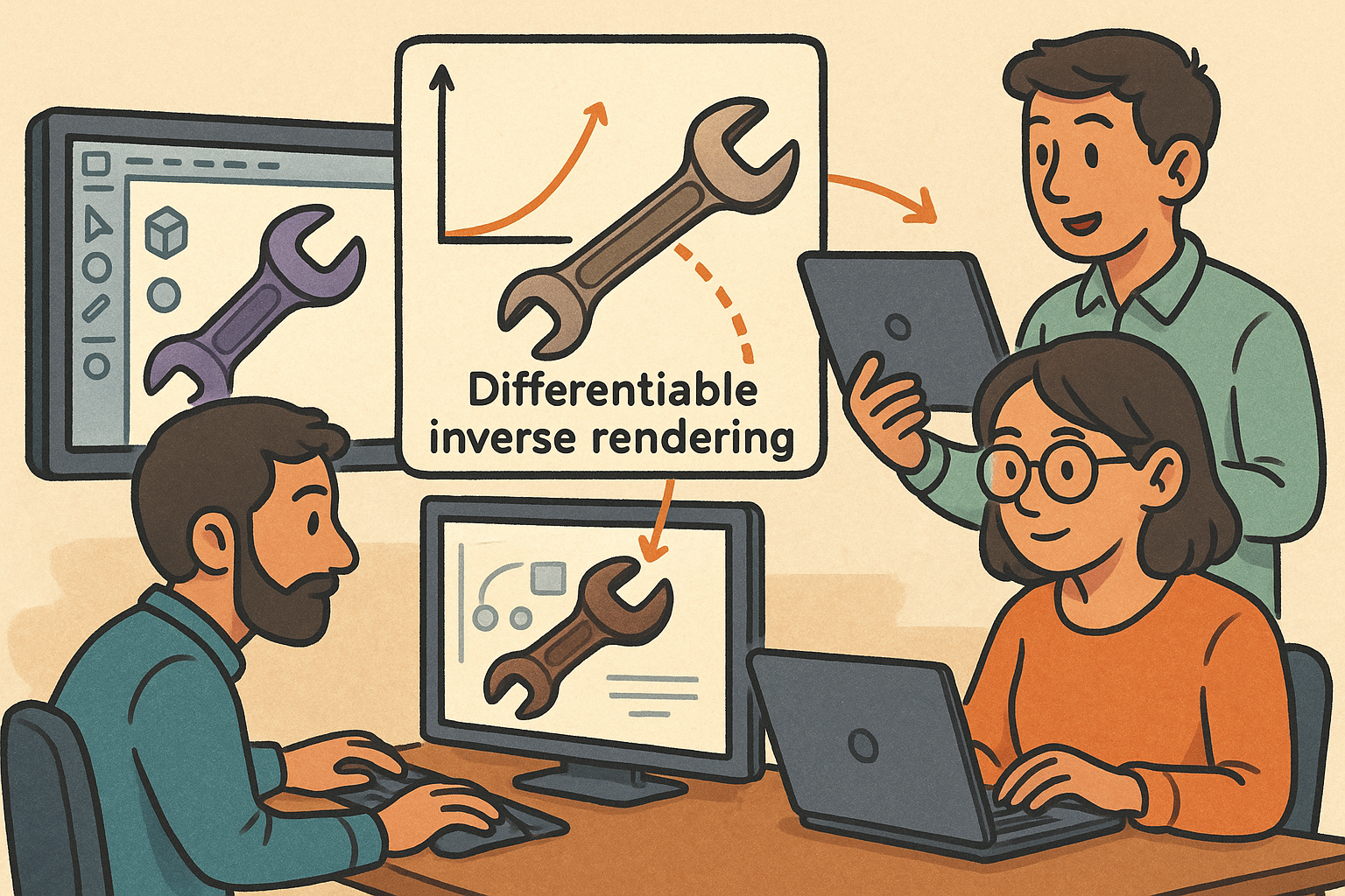
Designers have always sought renders that look indistinguishable from the real thing, but manual tweaking of sliders for albedo, roughness, metallic, and clearcoat has clear limits. The emerging approach replaces guesswork with **data-driven inverse rendering**, where we directly optimize **physically based material parameters** so the virtual outcome matches a target appearance under real or virtual lighting. The objective is straightforward: choose parameters—base color/albedo, roughness, metallic, index of refraction (IOR), anisotropy, clearcoat, subsurface scattering (SSS), and thin-film thickness—so CAD renders closely match calibrated photography or a well-defined reference, often measured using color-difference metrics such as **ΔE2000**. This shift matters because **PBR material models** have become unified across DCC and CAD tools, which standardizes the parameterization, and because **differentiable rendering** makes these parameters amenable to gradient-based optimization. As a result, what used to be multi-hour tuning sessions becomes a principled, repeatable process.

• Why now—model standardization: Disney/Principled BSDF variants and GGX microfacets are widely adopted, making parameter semantics portable across engines and file formats.
• Why now—computation: Modern GPUs plus autodiff frameworks (PyTorch, JAX) and libraries like nvdiffrast, PyTorch3D, redner, or Mitsuba/Dr.Jit deliver gradients at interactive to near-interactive speeds.
• Why now—workflow leverage: Teams already capture HDRIs, reference charts, and swatches; adding inverse rendering closes the loop from capture to validated material libraries.

Design workflow impact

Once gradients exist, the gating factor is no longer talent with a slider—it is simply whether the pipeline is calibrated. With cameras, lighting, and geometry aligned, a **gradient-based optimizer** can steer materials toward the image evidence, often converging within minutes. Across product categories—painted metal, textured plastics, fabrics, brushed aluminum, dielectrics under clearcoat—the technique directly supports known CMF criteria, including **ΔE targets** for color and perceived gloss under showroom lighting. More subtly, differentiable rendering enables perception-oriented goals: if a team defines a target impression (“crisper highlights,” “richer undertones”), the objective can be translated into a loss that biases parameters toward that perception while respecting physical plausibility. Where vendor files historically underperform due to generic defaults or missing layer interactions, inverse rendering makes vendor assets truly match what’s on the bench. It also streamlines material library curation, turning ad-hoc imports into calibrated, searchable assets with provenance.

• CMF convergence: Match paint, plastic, textile, and metal finishes to swatches or photography with explicit ΔE thresholds and gloss expectations.
• Visual verification: Tune vendor-supplied PBRs against measured BRDF/BTDF or consistent bench photos to eliminate persistent mismatches.
• Material library curation: Batch inverse-render turntable captures; export standardized, taxonomy-compliant assets to USD/MDL/MaterialX repositories.
• Perception-driven design: Optimize to maximize perceived quality under showroom HDRIs, translating subjective briefs into quantifiable objectives.
• Digital twins: Keep virtual appearance synchronized with as-manufactured variation by periodically re-fitting parameters from inline imaging.

What to optimize and how to constrain it

Optimization can target scalars, textures, or a mix. The low-dimensional route adjusts a handful of **scalar parameters** such as albedo tint, roughness, metallic, clearcoat weight, coat IOR, and thin-film thickness. In higher realism contexts, the pipeline estimates **full textures**: albedo maps, roughness maps, metallic masks, normal maps, and occasionally clearcoat-normal or thickness maps for layered stacks. For maximum fidelity, **lights, cameras, and environment maps** can be co-optimized with materials, though this requires careful priors to avoid trivial solutions (e.g., dimming lights instead of darkening albedo). The optimization is bounded by physics: energy conservation, plausible IORs, nonnegative reflectance, and manufacturability constraints (e.g., roughness and film thickness within achievable ranges). Texture regularizers suppress ringing and enforce spatial smoothness where appropriate, while preserving measured detail. With these constraints, the process remains stable and production-safe, enabling results that travel from fitting scenes into CAD viewports without surprises.

• Optimized variables: Scalar parameters (albedo, roughness, metallic, IOR, anisotropy, clearcoat), texture maps (albedo/roughness/normal), and sometimes lights/cameras/envmaps.
• Physical constraints: Energy conservation, Fresnel consistency, parameter bounds, and SSS positivity; enforce via clamping, barrier losses, and reparameterization.
• Regularization: Total variation (TV) for textures, Laplacian priors for normals, and low-pass priors for thin-film thickness to avoid color banding.
• Manufacturability: Soft constraints encoding supplier limits (e.g., gloss unit ranges, minimum coat thickness) so fitted values remain buildable.

Differentiable rendering toolbox and math essentials

Choosing a differentiation strategy

The choice between differentiable rasterization and differentiable path tracing depends on the observed phenomena and speed targets. Differentiable rasterization, as implemented in tools like **nvdiffrast** and **PyTorch3D**, excels at fast gradients for mostly diffuse and simple specular lobes. It is ideal for “on-the-fly” viewport tuning or rapid pre-optimization before handing off to a more accurate estimator. Conversely, **Monte Carlo differentiable path tracing**—in frameworks like **Mitsuba 3/Dr.Jit** or **redner**—captures the full richness of light transport: glossy interreflections, caustics, subsurface scattering, layered clearcoats, participating media, and thin-film interference. Because visibility and other discontinuities create gradient noise, mixed estimators combine **reparameterization gradients** for continuous effects with **score-function/REINFORCE**-style estimators for discrete events. The practical pattern is to start with rasterization for alignment and parameter warm-starting, then switch to path-traced gradients for accuracy-critical passes, allowing teams to balance throughput with fidelity without rewriting the objective or the optimizer.

• Differentiable rasterization: Fast, stable gradients, best for basecolor/roughness and simple reflections; validate with higher-accuracy methods before sign-off.
• Differentiable path tracing: Handles SSS, volumetrics, layered coats, glossy transport; needs variance reduction for stable gradients.
• Mixed estimators: Use reparameterization where possible; apply score-function estimators for visibility/shadow discontinuities; combine via multiple importance sampling.

Nondifferentiabilities and variance control

Silhouettes, hard shadows, and path discontinuities challenge gradient estimators, but practical techniques tame them. In rasterization, **soft visibility** and **edge sampling** smooth out boundary contributions while preserving geometry fidelity. In path tracing, one can switch between **primary-sample-space** and **path-space** gradient estimators depending on whether sampling PDFs or geometry changes dominate error. Crucially, gradient variance can be as significant as bias: variance-reduction strategies—MIS, stratification, low-discrepancy sequences, and path replay backpropagation—are as important as choosing the base estimator. Parameterization also matters: mapping roughness to **alpha = roughness²** stabilizes GGX derivatives, while optimizing strictly positive parameters (e.g., SSS scattering coefficients) in log space avoids invalid updates. Constraints can be handled via smooth barrier losses that guide the optimizer away from nonphysical regions without causing abrupt clipping. For textures, **TV regularization** encourages smoothness without over-smoothing fine detail, and a Laplacian prior helps normals remain integrable and consistent with observed shading cues.

• Soft visibility and edge integrals: Reduce gradient chatter at silhouettes; protect contours while enabling stable updates.
• Estimator domains: Choose between primary-sample and path-space gradients; combine with MIS to lower derivative variance.
• Reparameterization: Use alpha for GGX, log-space for positive parameters; apply bounded transforms with differentiable clamps or sigmoids.
• Regularizers: TV for textures, Laplacian for normals, and spectral smoothness penalties to tame thin-film oscillations.

Material models and spectra in practice

Production scenes rarely use a single lobe. The de facto **Disney/Principled BSDF** combines diffuse, specular GGX, clearcoat, sheen, and sometimes anisotropy; a differentiable implementation should expose gradients for each. Measured BRDFs—MERL, UTIA, or in-house gonioreflectometer scans—can be fitted to a lobe basis or used directly via differentiable interpolation, which preserves real-world features like backscatter and off-specular peaks. **Subsurface scattering** typically relies on diffusion or BSSRDF dipole models with differentiable parameters for scattering and absorption, plus surface roughness interactions for realistic glints on top of soft transport. **Thin-film interference** and layered stacks require differentiable Fresnel and thickness handling; while these give distinctive color shifts and angle-dependent highlights, they also introduce high-frequency spectral oscillations that can destabilize gradients in RGB-only pipelines. For color-critical work, **spectral fitting** produces more accurate ΔE under varied illuminants; when capture hardware is RGB-only, a learned illuminant-to-RGB mapping or camera spectral sensitivity approximation can bridge the gap, letting the optimizer operate in a pseudo-spectral space that still lands in expected CAD shaders. The key is consistency: the same BSDF and layer math used in rendering should be used for differentiation to avoid mismatched behaviors at validation time.

• Principled BSDF and GGX: Clear gradients for base/diffuse, specular, clearcoat, sheen, anisotropy; ensure energy conservation across lobes.
• Measured BRDFs: Basis fits or table interpolation with differentiable filtering; preserve non-GGX features of metals and fabrics.
• SSS and BSSRDF: Differentiable dipole/quantized diffusion models; couple with microfacet layers for realistic surface sheen.
• Thin-film and layers: Differentiable Fresnel and film-thickness; include spectral considerations to avoid RGB aliasing artifacts.
• Spectral vs RGB: Spectral optimization for ΔE accuracy; approximate camera/illuminant spectra if only RGB data is available.

Losses and objectives that behave

Loss design decides whether the optimizer learns the right perceptual trade-offs. **Photometric errors** (L1/L2) remain the backbone, but perceptual metrics like LPIPS align better with human judgments in texture-rich areas. For color-critical targets, **ΔE2000** or device-independent transforms (e.g., DEITP) help control hue and chroma errors under various illuminants. Multi-view and multi-light consistency prevents overfitting to a single setup, while view-specific weights can emphasize angles where appearance matters most (e.g., grazing highlights). Specular highlights and slight misalignments can inflate losses; **robust penalties** such as Charbonnier or Huber blunt outliers so the optimizer follows the median structure first, then tightens with a finer schedule. In texture fitting, **coarse-to-fine pyramids** mitigate local minima: fit low frequencies on downsampled textures, then progressively reveal higher-frequency detail. Multi-term objectives with schedulers let you sequence difficulty: lock down color first, then tackle roughness and anisotropy, finally addressing clearcoat and thin-film thickness. The result is a smoother training curve and fewer detours into visually unstable parameter regions.

• Core terms: L1/L2 photometric, LPIPS for perceptual quality, ΔE2000 for color accuracy, and SSIM for structural consistency.
• Robustness: Charbonnier/Huber to mitigate highlight clipping and small geometric misalignments.
• Consistency: Multi-view/multi-light constraints; view-dependent weights for critical grazing angles.
• Scheduling: Coarse-to-fine texture pyramids; staged emphasis from albedo to roughness to layered effects.

CAD workflow integration, performance, and validation

Pipeline patterns that fit real teams

To make **inverse rendering** usable in day-to-day CAD, the pipeline must mirror design realities: CAD geometry originates as B-Rep, materials must export to existing libraries, and the process should not disrupt review rituals. The common pattern starts with triangulating CAD to a stable tessellation and aligning cameras and lights via checkerboards or light probes. Materials begin with a principled PBR guess—often vendor-supplied—and the optimization targets a curated set of reference images or turntable captures. For viewport iteration, differentiable rasterization enables live tuning while showing error heatmaps or ΔE overlays. When accuracy matters—before catalogue imagery or executive reviews—the system switches to path-traced gradients and higher sampling, producing a calibrated asset that can be pushed back into USD/MDL/MaterialX libraries. Batch ingestion handles the long tail: a turntable or gantry captures multi-view datasets for many finishes in one go, and the system auto-fits, tags, and versions materials with provenance and metrics. In all cases, the optimized materials should round-trip cleanly back into the CAD renderer used by the team, ensuring that what was validated in fitting is what appears in standard scenes.

• Calibration mode: Inputs are triangulated CAD, initial PBR, measured HDRIs or lights, calibrated cameras, and reference imagery; outputs are fitted parameters exported to the CAD material library.
• On-the-fly tuning: Differentiable rasterization for immediate feedback; periodic path-traced validation to prevent drift.
• Batch asset ingestion: Turntable/gantry capture, auto-fit materials, enforce taxonomy and naming, and version control via PLM with USD/MDL/MaterialX.

Practicalities and optimizers that matter

Integration succeeds on the details. Geometry should be consistent: convert B-Rep to a tessellation that avoids frame-to-frame changes, fix seam issues, and stabilize tangents for normal mapping. UVs deserve special care: locking UVs keeps texture optimization well-posed; co-optimizing UV parameterization can be powerful but must be paired with strong regularizers to avoid foldovers. Lighting and cameras are frequently close but not perfect; jointly optimizing small deltas in HDRI rotation or intensity and camera intrinsics/extrinsics often pays off, especially if fiducials (Charuco boards, spheres) are in view. For optimizers, low-dimensional fits (a handful of scalars) respond well to **L-BFGS**, while **Adam/AdamW** shines for texture maps, particularly when combined with learning-rate schedules and early stopping. The UI should expose support tools—not just sliders, but live residual visualizations and convergence indicators—so designers can trust when the solution is “done.” The net effect is a workflow where fitting becomes a repeatable craft rather than an art project.

• Geometry: Stable tessellation, consistent tangents, robust UVs; optionally co-optimize UV unwrap with TV and ARAP-style regularizers.
• Lighting: Prefer measured HDRIs; allow small intensity/rotation corrections with priors to keep solutions realistic.
• Cameras: Optimize small pose/intrinsics deltas when fiducials are present; otherwise rely on pre-calibrated rigs and lock them in the optimizer.
• Optimizers: L-BFGS for low-D scalar fits; Adam/AdamW for textures; cosine or step LR schedules; early stopping based on validation views.

Performance, deployment, and quality assurance

Performance determines whether the technique is a lab curiosity or a daily habit. Mixed precision and **gradient checkpointing** lower memory footprints; sample reuse across iterations reduces per-step cost when the scene changes slowly. Multi-resolution textures and tile-based updates keep bandwidth bounded on large assets, while deterministic seeds stabilize regression testing. For path tracing, derivative variance dominates runtime; **guiding**, path replay backprop, and MIS ensure gradients reflect signal, not noise. Deployment-wise, wrapping the differentiable renderer as a service decouples CAD clients from the heavy compute, communicating via **USD/MaterialX/MDL** with cached irradiance/envmaps to avoid redundant work. The plugin UI should surface both control and confidence: sliders for loss weights, **live error heatmaps**, ΔE overlays, and a convergence bar that estimates remaining improvement. Validation closes the loop: fit on one HDRI, validate on others to catch overfitting; track ΔE2000 across charts, compare gloss units against gonioreflectometer readings, and verify BRDF lobe shapes by computing half-angle RMSE. Physical plausibility checks—energy conservation, IOR bounds, nonnegative textures—guard against visually plausible but nonphysical shortcuts. Finally, change management records inputs, seeds, software versions, and loss schedules so results are reproducible and improvable over time.

• Speed-ups: Mixed precision, checkpointing, sample reuse, multi-res textures, tiles; variance reduction via guiding and replay backprop.
• Deployment: Service-oriented renderer, USD/MaterialX/MDL I/O, cached envmaps/irradiance, pooled GPUs for batch jobs.
• Validation metrics: ΔE2000, gloss units vs gonioreflectometer, BRDF half-angle RMSE, SSIM/LPIPS for appearance fidelity.
• Cross-illumination: Fit on one HDRI, validate on several; check generalization and guard against scene-specific hacks.
• Plausibility: Enforce energy conservation, IOR bounds, nonnegative textures; flag violations automatically.
• Provenance: Record inputs, seeds, versions, and loss schedules; compare against hand-tuned baselines as a sanity check.

Conclusion

From principled fits to production assets

Differentiable rendering transforms appearance tuning from intuition-driven trial-and-error into **principled, data-driven optimization**. By aligning capture, modeling, and rendering under the same PBR semantics and exposing gradients for the full stack—materials, lights, and cameras—teams can fit **physically based material parameters** so virtual prototypes behave like their physical counterparts across lighting conditions. The practical recipe is not mysterious: pick the right estimator for the phenomena at hand (fast differentiable rasterization for previews, **path-traced gradients** for layered, glossy, and subsurface effects), design robust multi-term losses that encode color accuracy and perception, and keep the solution safely grounded with physical constraints and regularizers. Integrated thoughtfully—via **USD/MaterialX/MDL**, validated HDRIs, calibrated rigs, and reproducible pipelines—the approach accelerates CMF convergence, improves visual fidelity in review and marketing imagery, and builds material libraries that actually predict real-world appearance.

• What changes day to day: Designers focus on intent and acceptance criteria; the optimizer handles the heavy lifting, with live diagnostics indicating when further iterations are low value.
• What remains essential: Accurate capture, sensible priors, and validation across illuminants; gradients are only as trustworthy as the pipeline is consistent.
• Near-term opportunities: Better variance-reduced gradients for complex transport (caustics, volumetrics), spectrally accurate pipelines delivering ΔE guarantees, and tighter CAD plugins that mix real-time previews with batch-accurate refinement.

As tools and compute improve, fitting becomes less about clever workarounds and more about encoding the right objective. The reward is tangible: fewer surprises between design intent, vendor samples, and final product; faster cycles from brief to approval; and a reusable library of calibrated, layered materials that travel across scenes, teams, and platforms. The throughline is simple yet powerful—optimize what you show until it matches what you make—and with **differentiable rendering** now practical at studio scale, the gap between physical materials and CAD visuals finally closes in a measurable, repeatable way.