Your Cart is Empty
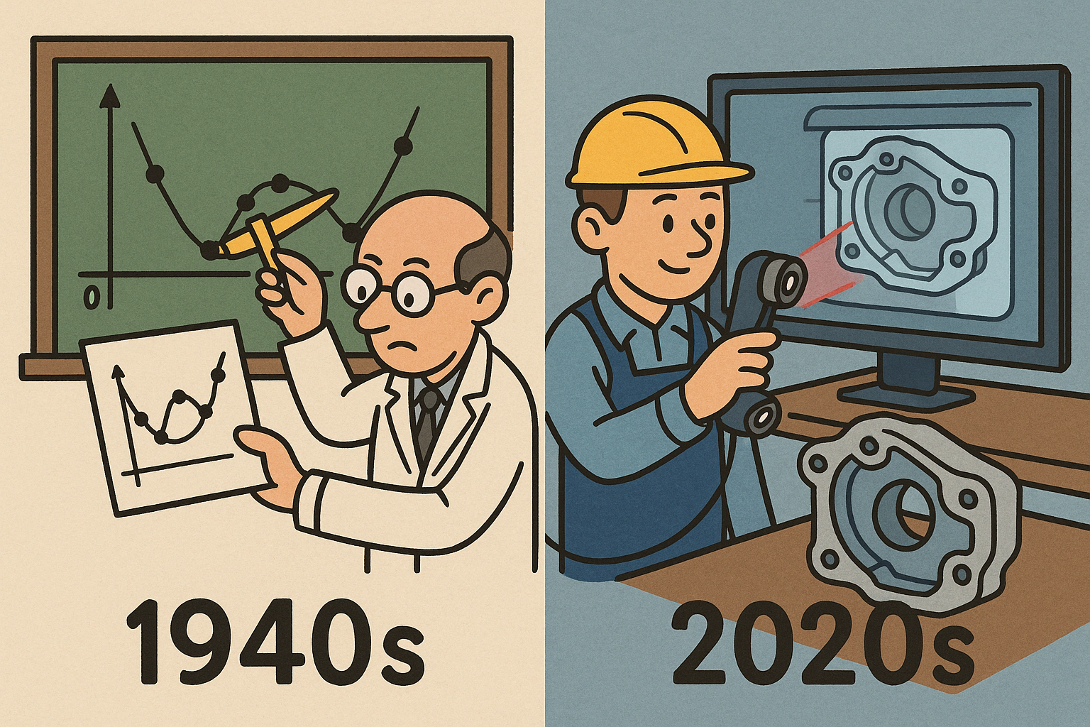
Design Software History: Scan Fitting: Mathematical Foundations and Industrialization (1940s–2020s)


Mathematical roots that made scan fitting possible (1940s–1980s)
From mechanical splines to polynomials
The path from shipwrights’ lead-weighted strips to the mathematics that power modern scan fitting runs through the decisive mid‑20th‑century formalization of splines. In 1946, I. J. Schoenberg reframed the carpenter’s spline as a piecewise polynomial with continuity constraints, a leap that replaced workshop intuition with analysis. A year later, in work often attributed to Isaac Jacob Schoenberg together with H. B. Curry, the Curry–Schoenberg B‑splines introduced stable, local basis functions whose compact support made computation and numerical robustness practical. With B‑splines, designers could shape with a handful of control points while algorithms guaranteed smoothness. By the 1960s, Pierre Bézier at Renault and Paul de Casteljau at Citroën independently institutionalized these ideas inside automotive styling. Bézier’s publicized curves and surfaces and de Casteljau’s recursive evaluation procedure (initially proprietary at Citroën) gave industry operators predictable tools that could be taught, repeated, and audited. Carl de Boor’s 1972 algorithm then provided a numerically stable method for evaluating nonuniform knot vectors, ensuring that local changes in control structure produced local changes in shape—a criterion essential for future fitting workflows where data irregularity is the norm rather than the exception. The conceptual through-line is clear: local control, partition of unity, and smooth join conditions made the spline not only a design primitive but a computationally sane building block. Those traits later enabled the jump from exact, designer-authored shapes to shapes inferred from imperfect measurements, because the same locality and stability that helped stylists in 1968 would help statisticians and geometricians confront noise in 1988.- B‑splines brought locality, stability, and reproducibility—ingredients missing in global polynomial fits prone to oscillation.
- Bézier/de Casteljau industrialized curve behavior, normalizing control polygon intuition across teams and decades.
- De Boor’s evaluation on arbitrary knot vectors underwrote adaptive refinement, a precursor to data-driven knot insertion in scan fitting.
From exact design to noisy data
As digitizers and coordinate measurement machines began returning imperfect samples, spline theory met statistics. The pivot came with penalized least squares and smoothing splines: Grace Wahba, between 1965 and 1975, framed spline estimation as the minimization of squared residuals plus a roughness penalty, while Christian Reinsch (1967) derived efficient solvers that balanced fidelity and smoothness via a single regularization parameter. This paradigm said, in effect, that the “right” shape is neither the one that passes exactly through every point (overfitting) nor the one that ignores data to remain elegant (underfitting), but the one that trades residual error against a fairness functional measuring curvature variation. That notion flowed directly into Computer Aided Geometric Design (CAGD), where Gerald Farin, Helmut Pottmann, and the duo Hoschek & Lasser elaborated energy minimization objectives—thin-plate energies, minimum variation of curvature, and integral measures of bending—that would later be embedded into reverse-engineering software as sliders labeled “smoothness” or “G2 quality.” The mathematics of Tikhonov regularization met the craft of surfacing: energy terms derived from second derivatives became dials that Class‑A modelers could tune while the solver suppressed wiggles introduced by scanner jitter or speckle noise. Crucially, these formulations are robust to nonuniform sampling—a practical necessity when a handheld scanner stares too long at a fillet and too briefly at a flat. By the late 1970s and early 1980s, the bridge had been built: estimation theory provided the statistical backbone; splines provided the geometric substrate; and optimization provided the means to marry them at industrial scale.- Smoothing splines = least squares fit + roughness penalty; a single lambda orchestrates the bias–variance trade‑off.
- Fairness energies (Laplacian/bi‑Laplacian, minimum variation) became proxies for perceived quality in Class‑A surfacing.
- Nonuniform sampling and outlier tolerance were addressed with weighted objectives and robust estimators, foreshadowing modern scan fitting.
NURBS unify precision and flexibility
The unification of precision geometry and freeform flexibility arrived with NURBS—Non‑Uniform Rational B‑Splines. In his 1975 PhD dissertation at Syracuse University, Kenneth Versprille codified rational B‑splines in homogeneous coordinates, showing that conic sections and other rational primitives sit naturally in the same framework as freeform B‑splines. This mattered because reverse engineering would need to honor exact circles, cylinders, and tori while also recovering sweeps and blends that defy closed form. Over the next two decades, Gerald Farin, and the duo Les Piegl and Wayne Tiller—culminating in “The NURBS Book”—standardized terminology, algorithms, and implementation practices so thoroughly that kernel vendors could interoperate. With rational weights, designers could express exact CAD intent; with nonuniform knots, they could concentrate degrees of freedom where features live. Early lofting workflows in automotive and aerospace—stations, cross‑sections, and ruled connections—foreshadowed scan‑driven patch networks: if you can drive surfaces from sparse, carefully chosen sections, you can also drive them from dense, measured sections cut through point clouds. Thus, by the mid‑1980s, industry had both the theory and the software vocabulary to represent the shapes a scanner would see decades later: spline spaces with controllable continuity, rational segments for exactness, and algorithms for evaluation, refinement, and conversion. The only missing piece was the robust machinery to turn unstructured, noisy measurements into parameterized surfaces—a gap the next wave of geometry processing and optimization would close.- Rational weights enable exact conics and quadric patches alongside freeform spans.
- Nonuniform, open knot vectors provide local refinement and predictable end conditions for patch trimming.
- Section-based lofting in CATIA/UNISURF era anticipated modern section‑driven fitting against scans and meshes.
Core algorithms for fitting splines to scanned data (1980s–2000s)
Getting data into one coordinate frame
Before any fitting can proceed, all measurements must inhabit a common frame. The breakthrough came with ICP (Iterative Closest Point), formalized by Paul J. Besl and Neil D. McKay in 1992. ICP alternates between establishing correspondences (closest points) and estimating the rigid transform that minimizes distances between matched pairs. It is deceptively simple yet profoundly effective, especially when combined with good initialization and rejection of spurious correspondences. Variants followed quickly: point‑to‑plane ICP replaces Euclidean distance with a first‑order approximation using target normals, greatly improving convergence on dense, locally planar scans; robust kernels downweight outliers; multi‑scale ICP coarse‑grains the geometry to widen the basin of attraction. In production, vendors complement ICP with marker‑based seeding, bundle adjustment across multiple stations, and moving‑horizon filtering for handheld trajectories. Alignment is not merely a preparatory step; it defines the tolerances within which all subsequent fitting will be judged. If your clouds are misregistered by a tenth, your spline fit cannot beat a tenth. Thus, ICP’s resilience and speed made it the unglamorous but essential workhorse in scan fitting pipelines throughout the 1990s and 2000s, bridging the world of raw digitizer output with the coordinate discipline demanded by CAD kernels and PLM vaults.- Core loop: assign correspondences → solve SE(3) via SVD or Horn’s quaternion method → iterate until convergence.
- Point‑to‑plane ICP accelerates convergence by minimizing normal‑projected distances; perfect for high‑density meshes.
- Robustness enhancers: trim worst residuals, use Huber/Tukey loss, and run from coarse to fine resolutions.
From raw points to fit-ready structure
Once registered, scans must be organized, denoised, and endowed with differential structure. David Levin’s 1998 formulation of Moving Least Squares (MLS) provided a principled way to estimate normals and a locally smooth approximation surface from scattered points. MLS fits a polynomial in a sliding window weighted by proximity, furnishing normals, curvatures, and even projections—indispensable for both fairing and oriented distance fitting. Meanwhile, surface reconstruction emerged as a means to impose topology: the seminal Hoppe et al. (1992) pipeline—normal estimation, signed distance function via an oriented point set, and isosurface extraction—gave scan data a coherent inside/outside and a mesh to which splines could later be conformed. In 2006, Michael Kazhdan, Matthew Bolitho, and Hugues Hoppe introduced Poisson reconstruction, formulating reconstruction as a global solution to a divergence equation; the result is watertight and robust to noise and incomplete coverage. With a surface in hand, segmentation and parameterization can proceed: curvature‑driven region growing isolates fillets, flats, and revolutes; cross‑field guided quadrangulation distributes parameter lines that respect principal curvature and intended patch layout; and conformal or authalic parameterizations map irregular regions to regular domains. All of this scaffolding transforms a cloud of points into a mesh with normals, regions, and parameter lines—a substrate friendly to spline fitting routines that expect well‑behaved samples, consistent orientations, and design‑meaningful patch boundaries.- MLS supplies normals and projections crucial for oriented distance objectives and fairing energies.
- Hoppe‑style signed distance fields and Poisson reconstruction deliver watertight meshes and inside/outside consistency.
- Segmentation + cross‑field quadrangulation = spline‑ready charts whose parameter lines echo curvature and features.
Curve and surface fitting primitives
With structure in place, the fitting proper begins. Classical B‑spline and NURBS fitting typically starts by parameterizing samples—using chord‑length or centripetal schemes for curves and surface parameterizations pulled from the mesh for patches—then solving a least‑squares system for control points. To achieve a target tolerance with minimal complexity, adaptive strategies insert and remove knots based on residuals: de Boor’s theories on spline spaces provide the backbone; Les Piegl and Wayne Tiller popularized practical algorithms that split spans where errors concentrate and prune where control points contribute little. Weighting combats nonuniform sampling; robust estimators like Huber or Tukey suppress outliers; and, for oriented geometry, normals enter the objective, minimizing distances along normals rather than naïve Euclidean norms. On top of geometric fidelity, professional surfacing chases Class‑A quality: fairing energies—discrete Laplacian or bi‑Laplacian, minimum variation of curvature—are imposed as soft constraints or penalties, a practice long ingrained in ICEM Surf and Alias AutoStudio communities. The result is a saddle point between error and elegance: deviations lie within scanner tolerance while curvature plots remain monotone and transitions achieve G2 continuity. Iteration is inevitable: adjust parameterization, reinject knots, reweight residuals, and re‑fair until diagnostic plots—zebra stripes, highlight lines, and deviation heatmaps—agree with the engineer’s eye.- Start with chord‑length/centripetal parameterization; refine with reparameterization when residuals show drift.
- Adaptive knot insertion/removal maintains tolerance with the fewest DOFs, avoiding overfit ripple.
- Fairing via Laplacian/bi‑Laplacian energies delivers G2 “Class‑A” smoothness aligned with aesthetic criteria.
Alternatives and complements to spline fitting
While NURBS dominate editable CAD, alternatives enrich the toolbox, especially in reconstruction and deformation contexts. Radial Basis Functions (RBFs), introduced by Rolland Hardy (1971) and connected to variational splines by Duchon (1977), define smooth implicit surfaces from scattered points with theoretically elegant interpolation/smoothing trade‑offs; their thin‑plate spline specializations, popularized by Fred Bookstein (1989), minimize bending energy and excel at global, low‑frequency shape capture. These implicit models serve as intermediate representations for meshing, offsetting, and collision‑free projection back onto measured geometry. In parallel, subdivision surfaces delivered smoothness over arbitrary topology; and with Thomas W. Sederberg and colleagues’ 2003 introduction of T‑splines, local refinement arrived without the topological baggage of tensor‑product NURBS. T‑splines allowed T‑junctions in control grids, aligning modeling complexity with geometric complexity—a gift to reverse‑engineering workflows that must densify only where scans demand it. In practice, teams combine these methods: an RBF or Poisson implicit smooths and fills; quadrangulation yields charts; T‑spline or NURBS patches are then fit with local refinement and fairness penalties. The philosophical point is that scan fitting is not monotheistic: it recruits the right representation at the right moment—implicit for watertightness, subdivision/T‑splines for flexibility, and NURBS for kernel‑grade exactness and downstream manufacturing.- RBFs/thin‑plate splines give global, smooth implicits ideal for hole filling and pre‑fairing.
- Subdivision and T‑splines provide local refinement and topology freedom beyond tensor‑product grids.
- Hybrid pipelines exploit implicits for robustness and NURBS for precise, editable deliverables.
Industrialization: software stacks, people, and practice (1990s–2020s)
Dedicated reverse-engineering tools
The leap from research prototypes to shop‑floor reliability came via specialized tools and the entrepreneurs behind them. Geomagic, founded by Ping Fu and Herbert Edelsbrunner, democratized scan‑to‑CAD with workflows that wrapped ICP, hole filling, mesh optimization, and surface fitting behind a user interface that spoke engineering language. INUS Technology’s RapidForm (later acquired by 3D Systems) pioneered parametric “feature transfer” that reconstructed editable sketches, extrusions, and revolves directly from meshes—a bridge between raw data and history‑based CAD. Paraform, an early Class‑A surfacing tool, targeted automotive studios with curvature‑tooling that understood highlights and G2+ continuity. InnovMetric’s PolyWorks|Modeler stitched metrology and modeling into one environment; Creaform’s VXModel linked handheld scanners to downstream CAD; and GOM—now in the ZEISS ecosystem—connected optical metrology to CAD validation via deviation maps and inspection templates. Consolidation ensued: Nikon acquired Metris in 2009 to fuse measurement and design verification; Dassault Systèmes acquired ICEM Surf in 2007 to anchor high‑end surfacing within CATIA; and 3D Systems brought RapidForm (2012) and Geomagic (2013) under one roof, assembling a stack from scan capture to manufacturing file. These moves signaled maturity: reverse engineering was no longer a niche task but a production capability used to repair tooling, onboard supplier geometry, and archive as‑built condition for regulated industries.- Geomagic: accessible scan‑to‑surface flow with robust mesh healing and NURBS generation.
- RapidForm/Design X: parametric feature extraction that lands inside mainstream CAD histories.
- PolyWorks, VXModel, GOM/ZEISS: tight coupling of metrology, fitting, and inspection with enterprise reporting.
CAD-integrated modules and workflows
Major CAD platforms absorbed reverse‑engineering mechanics to keep users in‑context. Dassault Systèmes embedded Digitized Shape Editor and Quick Surface Reconstruction in CATIA so that automotive and aerospace teams could align, filter, and surface scans without leaving V5/V6; Siemens NX added Reverse Engineering and later Convergent Modeling to blend mesh and B‑rep operations; PTC introduced Creo REX (Reverse Engineering Extension) to promote direct conversion of polygonal data to editable features; and SolidWorks shipped ScanTo3D to address prototyping needs inside SMB workflows. On the Class‑A side, Alias AutoStudio (Autodesk) and ICEM Surf remained the gold standards for curvature and highlight analysis; their influence on best practices—zebra stripes, curvature combs, min‑variation fairing—permeates all scan‑driven surfacing. Autodesk’s acquisition of T‑Splines (2011) filtered into Fusion 360’s “Form” workspace, bringing local refinement and sculpting ergonomics to engineering audiences and making it plausible to start from an imported mesh and end with editable, production‑oriented NURBS or T‑splines. Meanwhile, Rhino (Robert McNeel & Associates), with its robust NURBS core and vibrant plugin ecosystem—RhinoResurf, legacy VSR tools later reborn as Autodesk’s VRED/Alias adjacencies—democratized advanced surfacing for consultancies and small shops. The net effect was cultural as much as technical: scan‑aware tools moved from specialist stations to every designer’s desktop, and the language of residuals, fairness, and G‑continuity became shared currency across departments.- CATIA DSE/QSR, NX Reverse Engineering, Creo REX: integrated scan alignment and NURBS surfacing inside parametric CAD.
- Alias/ICEM: sustained emphasis on G2/G3 continuity and highlight‑based evaluation for Class‑A deliverables.
- Rhino + plugins: affordable entry with pro‑grade NURBS and mesh tools that shortened the learning curve.
Under-the-hood kernels and libraries
Behind every user interface lie geometry kernels and numerical libraries that make fitting scalable and interoperable. Parasolid (Siemens), ACIS (Spatial/Dassault Systèmes), and CGM (Dassault Systèmes) provide industrial‑strength NURBS operators—intersection, projection, offsetting, trimming—that must behave deterministically across edge cases. SINTEF’s SISL, driven by Tore Dokken and colleagues, quietly powers spline evaluation, intersection, and fitting routines inside many commercial and academic codes, its provenance visible in function names that echo Farin/Piegl‑Tiller conventions. OpenCASCADE offers open‑source BSpline construction and fitting utilities (e.g., GeomAPI_PointsToBSpline), inviting customization and auditability. For upstream processing, CGAL supplies surface reconstruction and segmentation primitives, while the Point Cloud Library (PCL) gives ICP, MLS, and filtering staples. The numerical muscle—SuiteSparse (Timothy Davis) for sparse factorizations and Ceres Solver (Google) for robust, large‑scale non‑linear least squares—turns objective functions with millions of residuals into overnight or even real‑time results. In modern stacks, GPU‑accelerated nearest neighbor search, robust loss functions, and automatic differentiation bridge geometry and optimization, allowing developers to add fairness penalties and constraint Jacobians with minimal boilerplate. The reliable interplay between kernels, libraries, and solvers—developed over decades of bug fixes and edge‑case handling—is why today’s scan‑to‑CAD tools can promise millimeter tolerances on billion‑sample captures without blinking.- Parasolid/ACIS/CGM: deterministic NURBS operators and trimming that downstream manufacturing can trust.
- SISL and OpenCASCADE: accessible spline fitting and evaluation blocks reused across products and research.
- CGAL/PCL + SuiteSparse/Ceres: geometry processing meets scalable optimization under robust loss functions.
A canonical scan-to-spline pipeline (as practiced)
A mature shop tends to follow a disciplined, instrument‑agnostic pipeline whose steps have been hardened by thousands of parts. It usually begins with acquisition—structured light, laser line, or computed tomography—followed by target‑based pre‑alignment and ICP registration across views. Next comes denoising and normal estimation, often via MLS, with outlier culling and resampling to obtain uniform coverage. A surface is reconstructed—Poisson for watertightness or Hoppe‑style signed distance for editability—and decimated to a working resolution. Segmentation isolates primitives (planes, cylinders, cones, tori) and freeforms; parameterization over freeform regions sets up NURBS/T‑spline charts. Curve networks are extracted from natural sections and feature lines, then used to seed patch boundaries. Initial fits solve a weighted least‑squares problem with centripetal parameterization; adaptive knot insertion pursues the target tolerance while fairing energies suppress ripple. For edges and transitions, continuity constraints enforce G1/G2 across patch seams; for trims, robust projection and reparameterization avoid slivers. Validation is treated as first‑class: deviation heatmaps, max/mean residual statistics, and highlight lines diagnose both geometric error and aesthetic quality. Round‑trip tests—export to the target kernel and reload—verify that tolerances survive translation. Finally, the model is committed to PLM with metadata: scanner settings, fitting parameters, and inspection templates so downstream QA can reproduce comparisons.- Acquire → register → denoise → reconstruct → segment/parameterize → extract curves → fit/fair → validate → export.
- Deviation heatmaps and G‑continuity checks guard both tolerance and visual smoothness.
- Export paths honor kernel idiosyncrasies to preserve trims, tolerances, and continuity.
Conclusion
Where the threads meet
Spline fitting for scanned data sits precisely at the seam between three traditions: the analytic rigor of CAGD, the pragmatism of statistical estimation, and the algorithmic inventiveness of geometry processing. From Schoenberg’s formalization of splines and de Boor’s algorithms, through Bézier and de Casteljau’s industrial curve control, to Versprille’s rational unification, the geometric language matured to represent both elegance and exactness. Concurrently, Wahba’s and Reinsch’s penalized least squares gave a vocabulary to arbitrate between fit and fairness, while Farin, Pottmann, and Hoschek & Lasser translated that vocabulary into surface energies that stylists and engineers could tune. Geometry processing then supplied the missing connective tissue: ICP for alignment, MLS for normals and projection, Poisson for watertightness, segmentation and parameterization for patch‑readiness. The arc of the field, seen across decades, is one of convergence: mature theory enabling robust algorithms, and robust algorithms packaged into dependable software—Geomagic/Design X, Alias/ICEM, CATIA/NX/Creo/Rhino—that has normalized scan‑to‑CAD across industries. The remarkable part is how modular the stack remains: swap in a different normal estimator, a different fairing penalty, or a different solver, and the pipeline still holds, testifying to the depth of the foundations. That modularity will be the springboard for the next advances as data volumes balloon and expectations shift from hours to minutes.- CAGD theory: B‑splines/NURBS, continuity, fairness functionals, and exact rational primitives.
- Statistical estimation: robust, weighted, and penalized least squares to tame noise and outliers.
- Geometry processing: registration, reconstruction, segmentation, and parameterization at scale.
Enduring and emerging challenges
Despite maturity, hard problems remain in the gap between “as‑scanned” fidelity and “as‑designed” intent. Automating patch layout while preserving feature sharpness is notoriously delicate: algorithms read curvature and symmetry, but intent lives in undocumented constraints like draft angles, tooling pull, and highlight flow. Achieving Class‑A smoothness with low model complexity calls for smarter refinement—hierarchical B‑splines, LR‑splines, and T‑spline‑style locality—without exploding parameterization seams or introducing T‑junction artifacts when exported to conservative kernels. Watertightness with high‑order continuity is also demanding: trims and joins must negotiate tolerance stacks from scans, fits, and kernel booleans. Scale, too, pushes boundaries: billion‑point captures tax nearest neighbor search, memory, and solver bandwidth; distributed, out‑of‑core strategies and GPU‑accelerated linear algebra are becoming mandatory. Finally, representation bridging is unfinished business: mapping from meshes—and now neural/implicit fields—to editable NURBS/T‑splines with guarantees on deviation and continuity is still more art than science. Solvers can certify residuals, but certifying design intent remains cognitive. The industry’s next gains will come from making that cognitive load legible to algorithms without surrendering the designer’s final say.- Automated patch layout that encodes design intent, symmetry, and manufacturability constraints.
- Local refinement (hierarchical/LR‑splines) without topological baggage or kernel incompatibility.
- Scalable solvers and data structures for trillion‑sample regimes and streaming capture.
- Bridging meshes/implicits to NURBS/T‑splines with certified tolerance and continuity.
What comes next
The next chapter will entwine differentiable optimization and data‑driven perception with classical spline theory. Differentiable renderers and simulators make it straightforward to backpropagate through registration, parameterization, and even trimming, letting us optimize control points, knots, and weights end‑to‑end under objectives that include photometric agreement, normal alignment, and fairness. At the same time, AI‑driven segmentation can propose patch layouts, extract feature lines, and predict primitive classes from partial scans, seeding the optimization with intent‑aware structure. Expect pipelines where ICP, MLS, and Poisson become learnable modules with priors tuned to the object class—turbomachinery, orthotics, body panels—so that the initial guess is already close to a manufacturable surface. On the solver side, sparse autodiff and second‑order methods will shrink solve times from hours to minutes for million‑DOF problems, while GPU‑resident nearest neighbors erase transfer bottlenecks. The endpoint is near‑real‑time scan‑to‑CAD that respects both tolerance budgets and the aesthetics long guarded by master surface modelers: highlight lines that sing, curvature that glides, and topology that edits gracefully six months later. As ever, the winners will be those who blend the old and the new—Schoenberg’s rigor with modern autodiff, Farin’s fairness with learned priors, and kernel‑grade robustness with studio‑grade sensitivity—turning a noisy point cloud into a surface that is not only accurate, but also right.Also in Design News